
I see that often many users have issues with managing lists of values and translating them to unique/distinct lists where values do not repeat themselves. There are many way to tackle this problem and you would be surprised that there even is a formula to handle this task. Let’s dive into this subject.
What we have (unsorted list) Vs. What we want (distinct list of sorted values)
Let’s assume a simple table of data. Where column A is full of repeating Names and column B is a list of corresponding values. We will be working on this data set through out this post. This data set is a typical example of the issue we often have with repeating rows of indistinct data. What we will want to do is to somehow summarize this table with a list of distinct Names and aggregated Values.
What we have
Let’s assume we have a simple table of Names and Values. What we will want to do is to somehow summarize this table with a list of distinct Names and aggregated Values.
| Name (A column) | Value (column B) |
|---|---|
| Tom | 60 |
| Matthew | 98 |
| James | 19 |
| John | 16 |
| Matthew | 45 |
| John | 26 |
| John | 70 |
| James | 60 |
What we want
The result of this operation should look somewhat like this:
| Name | Value |
|---|---|
| James | 79 |
| John | 112 |
| Matthew | 143 |
| Tom | 60 |
Now let’s familiarize with 2 approaches to this issue.
Method 1: Distinct column using a PivotTable
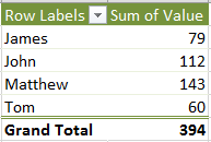
The most obvious solution is of course to create a PivotTable from this data set. All we need to do is add the Names as ROWS and Values as VALUES to the Pivot to get a simple summary with the exact data we need. See below:
Method 2: Distinct column using Array Formulas
Now putting aside the obvious, in some cases Pivots are not the answer. Especially if we don’t want to use VBA Macros and want to create a dynamic table which will simply update itself with the latest Values and Names.
Provide list of distinct Names
The first issue which we stumble upon is to somehow produce a list of distinct Names. At first this may seem impossible to be done by a Excel function. Fortunately again Array Formulas can come in handy in this task. This site features the elegant solution to this problem which I will try to explain in much detail.
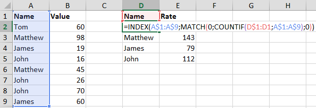
To provide a list of distinct Nameswe must use the following formula:
=INDEX(A$1:A$9;MATCH(0;COUNTIF(E$1:E1;A$1:A$9);0))
This is the final outcome when we hit CTRL+SHIFT+ENTER to make the formula an Array Formula and drag it down:
Now let’s ponder for a second on how the formula works as it might not be so straightforward as it seems:
'Gets an item from A$1:A$9 with an index provided by the MATCH function
=INDEX(
       A$1:A$9;
'Find value "0" in the column of value provided by the COUNTIF function
       MATCH(
            0;
'Returns an array. Count items from array A$1:A$9 if they are provided
'on the E$1:E1 list
            COUNTIF(
'Notice that this list has only 1 static item. The first item is the
'anchor, however, the second item will move to include all rows above
'the current one
                   E$1:E1;
                   A$1:A$9
                   );
            0)
      )
The exciting thing is how the MATCH function is used above. Usually the MATCH function is provided with a range of cells. This time, however, we are providing it with an array being the result of the COUNTIF function. What the MATCH function does is search for the first item resulting from the COUNTIF that has 0 counts i.e. it has not yet been provided in the list.
Now the formula will start producing #N/A errors when dragged beyond the number of distinct elements in the Names columns. You can correct this by wrapping it with a IFERROR function:
=IFERROR(
        INDEX(A$1:A$9;MATCH(0;COUNTIF(E$1:E1;A$1:A$9);0))
        ;"")
Sort the list of distinct Names
Now that we know how to provide a list of distinct names we still need to make sure that the list is sorted alphabetically else it will be provided in the same order as the items on the initial list. Here we need again to resort to Array Formulas to help us with this tasks.
Let’s start with explaining how to get the index of each name (concept from Chandoo.org):
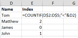
Notice the code in column E:
=COUNTIF(D$2:D$5;"<"&D2)
What we are doing is counting, for each distinct name, the number of items alphabetically of lower lexicographical value than our the current Name (D2).
Let’s now consider an Array Formula based on this:
=COUNTIF(D$2:D$5;"<"&D$2:D$5)
If we hit F9 we will see that an Array Formula would evaluate to:
={3;2;0;1}
This is the correct sequence of our list of distinct items.
If we combine this with an INDEX-MATCH combo we can iterate through this sequence:
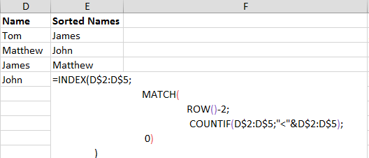
'Gets an item from D$2:D$5 with an index provided by the MATCH function
=INDEX(D$2:D$5;
'Find value of the current ROW-2 (this is simply to sequence through
'the arrary) in the column of value provided by the COUNTIF function
               MATCH(
                    ROW()-2;
'Evaluates to {3;2;0;1} - this is the correct sequence of our distinct
'array of Names
                    COUNTIF(D$2:D$5;"<"&D$2:D$5);
                    0)
      )
Summary
Now to summarize what we have.
- First, we provided the distinct list of Names in column D
- Secondly, we provided a separate column which sorts the distinct Names in column D
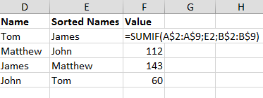
- Lastly, if we add a simple SUMIF function as shown below we can sum all values for each distinct Name in the Names column
Next Steps
Check out other similar posts:
EXCEL: Dynamic row numbers
EXCEL: 10 Top Excel features
EXCEL: Split columns on any pattern


")